The Most Important Excel Formulas While Education

Excel offers thousands of built-in functions to make your work or study much easier. It is enough to know only a part of them to save yourself time when processing data and building reports. Let’s take a look at the top 10 basic Excel functions, which are most often used during study or work in Higher Education Institutions. Some certain formulas might be familiar to you and you might have even used them, as some of them are widely used in teaching students of economics and computer science degrees.

Top 10 Excel Formulas for Studying

Important: The calculated results of formulas and some Excel worksheet functions may be slightly different between Windows x86 or x86-64 computers and Windows RT ARM computers.

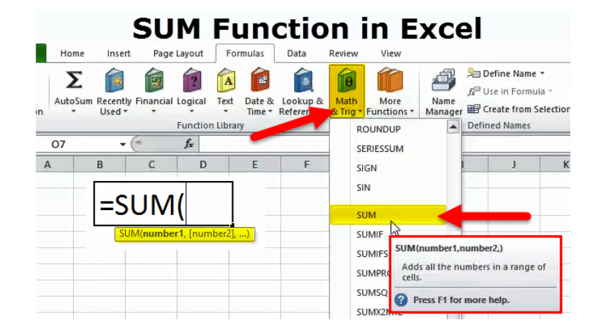
#1. SUM

Syntax: =SUM(number1;[number2];…), where number1 is a required argument.

The function makes it possible to find the sum of individual numeric values, ranges, cell references with numeric values, or the sum of all these 3 types. Often used in summarizing rows or columns when generating reports.

If one or more cells in a range of cells are blank or blank or contain text instead of a number, Excel ignores those values ​​when calculating the result.

The SUM function can also use mathematical operators such as (+, -, / and *)

Formulas do not update links when inserting rows or columns

When you insert a row or column, the formula does not update – it does not include the added row, while the SUM function will automatically update (as long as you have not gone beyond the range referenced by the formula). This is especially important when you expect the formula to update but it doesn’t. As a result, your results remain incomplete, and this may not be noticed.

#2. COUNT

Syntax: = COUNT(value1;[value2];…), where value1 is a required argument.

With this function, you can count cells that contain only numeric values ​​in the argument list. Often used in calculating averages when using the AVERAGE function in Excel is impractical. The following formula returns the number of cells in the range A1:E4 that contain numbers.

If all these formulas seem to be too complicated, try to use a service like Edubirdie where you can find help with your subjects like mathematics or economics. And it does not matter whether you are in school, college or university – studying math can be challenging at any age. By reading related essays on the Internet before exams, you can greatly improve your knowledge.

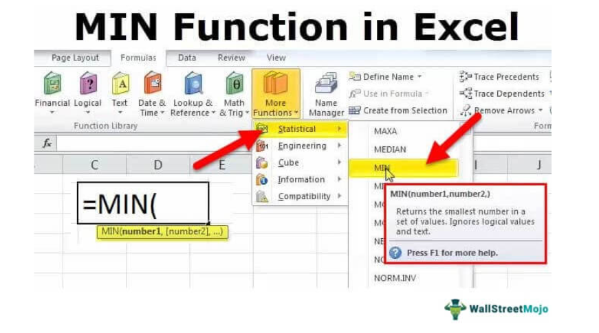
#3. MIN

Syntax: =MIN(number1;[number2];…), where number1 is a required argument.

The function allows you to find the minimum numeric value in the specified list of arguments. Often used in the construction of financial statements, when you need to determine the start date of the reporting period, the minimum purchase receipt, and other parameters.

Other important points relate to this formula. Arguments can be either numbers or names containing numbers, arrays, or references. Boolean values and textual representations of numbers that are directly entered in the argument list are taken into account. If the argument is an array or a reference, then only numbers are considered. Empty cells, booleans, and text in an array or reference are ignored. If the arguments do not contain numbers, the MIN function returns 0.

#4. AVERAGE

Syntax: = AVERAGE (number1;[number2];…), where number1 is a required argument.

With this function, you can find the arithmetic mean of individual numeric values, ranges, cell references with numeric values, or the average of these 3 types. Calculated by summing all the numbers and dividing the sum by the number of the same numbers. Text and Boolean values ​​in the range are ignored. This formula can be used for those students who need to know the average of their grades to apply for some types of scholarship.

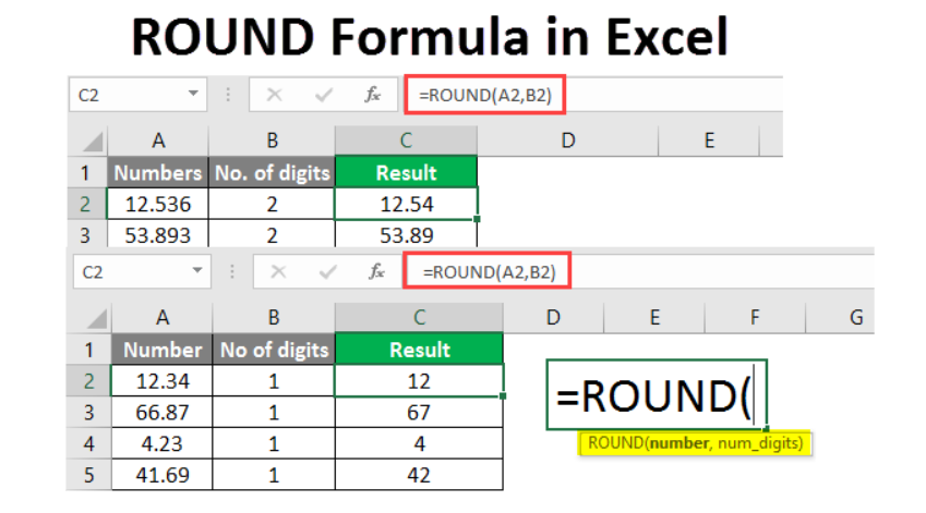
#5. ROUND

Syntax: = ROUND(number; number_digits), where number is the argument.

num_digits — to which digit the number is rounded.

The ROUND function is used to round real numbers to the required number of decimal places and returns the rounded value according to the mathematical rounding rule.

If the number of digits is greater than 0, then the number is rounded to the specified number of fractional digits. If the number of digits is 0, then the number is rounded up to the nearest integer. If the number of digits is less than 0, then the number is rounded to the left of the decimal point. To always round up by modulo, write the function ROUNDUP.

#6. IF

Syntax: =IF (logical_expression, value_if_true, value_if_false), where:

• boolean_expression is the condition that the operator checks for.
• value_if_true – if the condition is true, this value will be returned.
• value_if_false – if the condition is false, this value will be returned.

This function is one of the most famous in working with Excel. It checks numbers and/or text, functions, and formulas. When the values ​​meet the specified condition, a record appears from the “value_if_true” field, if they do not answer – “value_if_false”. Often used to distribute expressions into categories, and groups.

The function supports the use of comparison operators: = (equal to), < (less than), <= (less than or equal to), > (greater than), >= (greater than or equal to), <> (not equal to). This function is also often used in conjunction with the logical operators AND, OR.

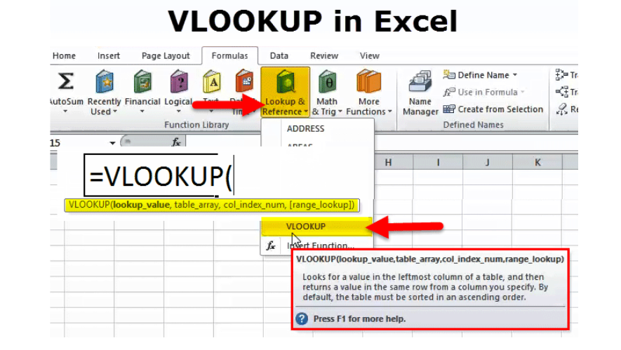
#7. VLOOKUP

Syntax: = VLOOKUP (lookup_value; table; column_number; [range_lookup]), where:

• lookup_value is the value to be found in the data column. Arguments can be numeric or text. The value you are looking for must be in the leftmost column of the range of cells in the specified table.
• table – a reference to a range of cells. The left column searches for the desired value, and the corresponding value is displayed from the columns to the right. The left column is also called the key column. If the table does not contain the value you are looking for, a #N/A error will be returned.
• column_number is the number of the table column according to which you want to display the result.
• [range_lookup] is an optional argument. It takes two values: TRUE and FALSE. TRUE is the default and the function assumes that the left column of the table is sorted in ascending alphabetical order. If this argument is TRUE, the function searches for the value closest to or the same as the searched value, FALSE searches for a 100% match with the searched value.

This is a feature that will make it easier to work with large data arrays and multiple tables. It will be useful if you need to pull up a column corresponding to the criterion from another table (for example, group, category).

#8. IFERROR

Syntax: = IFERROR (value; value_if_error), where:

•       value – the argument that is checked for an error
•       value_if_error – The value that is returned if an error occurs.

This function tests the argument against the error values ​​#N/A, #VALUE!, #REF!, #DIV/0, #NUM!, #NAME? or #EMPTY!. If the expression in the cell being tested contains an error, the function will return the value that is defined in that case. If there is no error, the result of calculations or cell data. Often used when dividing by zero.

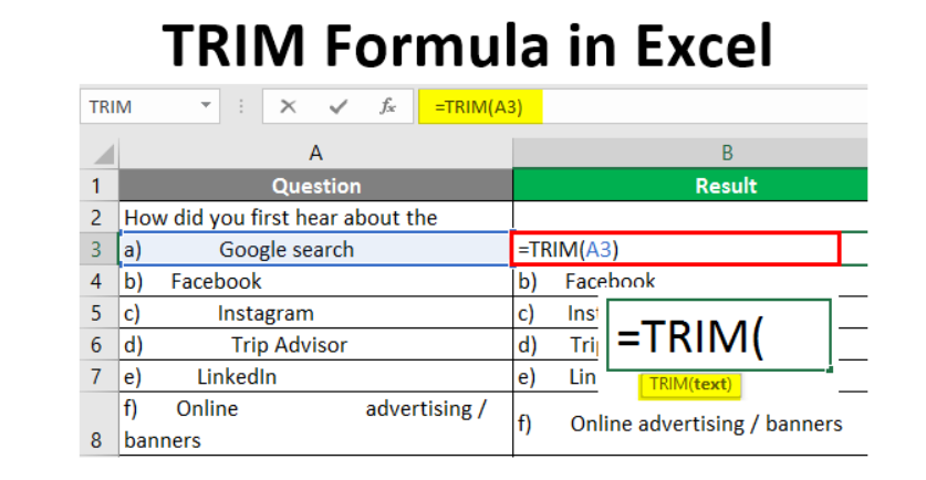
#9. TRIM

Syntax: = TRIM(text), where text is the text value from which to remove extra spaces.

This function is used to process texts from different sources. When there are extra spaces in these texts, they are removed.

Using the function, you can remove extra spaces from the text (character code – 32). In some cases.

The TRIM function cannot remove the non-breaking space (value 160) that is commonly used as an HTML entity in web pages – this can be useful for those who study programming languages. You can manually remove the non-breaking space character using the SUBSTITUTE function.

You can apply the TRIM function to extra spaces between words in the text. You can use the TRIM function to remove all spaces from the beginning and end of a text string.

#10. CONCATENATE

Syntax: CONCATENATE(text1, [text2], …), where text1 is a required argument.

To combine values ​​from different cells into one, use the CONCATENATE function. You can also use the analog – & (ampersand). The function is often used to combine data from multiple columns.

The CONCATENATE function combines up to 255 text lines into one. The elements to be merged can be text, numbers, cell references, or a combination of these elements. For example, if cell A1 of a worksheet contains the names of people who live with you on campus, and cell B1 contains their last names, you can use this formula to combine the two values in the third cell.

Conclusion

These were the most popular formulas to use for making the education process easier. By learning at least half of them, no math course or even integrals will frighten you! But there are more than just 10 formulas, so feel free to google any other formulas for your needs. Be sure that teachers will absolutely appreciate your deep knowledge of formulas, especially while online studying.

The Excel program is also actively used for planning budgets, which is critical for students, and for many other life tasks that a modern person sets for himself every day. The skills of working in this program help to quickly, easily and efficiently cope with a large number of numbers!